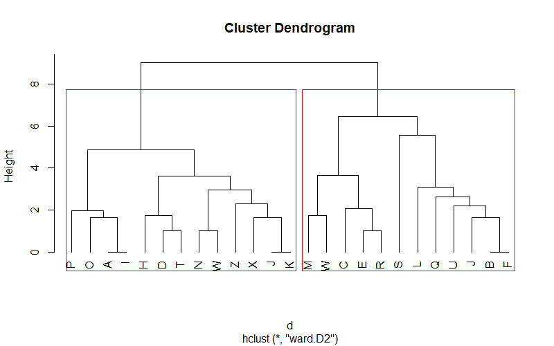
クラスター分析とデンドログラムの表示
library(readr)
library(dplyr)
library(magrittr)
library(reshape2)
library(ggplot2)
library(fpc)
# データの概要
   label item1 item2 item3 item4 item5 item6 item7 item8 item9 item10
1  A     5     5     5     5     5     5     5     5     5     5
2  B     5     4     4     4     4     4     4     4     3     3
3  C     5     5     5     5     5     5     5     4     5     1
4  D     5     5     5     5     5     5     5     3     4     3
6  E     5     5     5     5     5     5     5     5     3     1
7  F     5     4     4     4     4     4     4     4     3     3
# Euclidean Distance
d <- dist(dat[, -1], method = "euclidean")
# Hierarchical Clustering with Ward Method
cluster <- hclust(d, method = "ward.D2")
# Dendrogram
plot(cluster, labels = dat$label, hang = -1)
# k = nのクラスター数で囲いを入れる
rect.hclust(cluster, k = 2, border = "red")
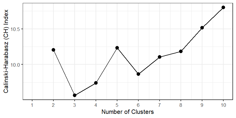
クラスター数の決定
##Calinski-Harabasz (CH) index(Pseudo F)
# total sum of squares
totss <- function(dmatrix){
  grandmean <- apply(dmatrix, 2, FUN = mean)
  sum(apply(dmatrix, 1, FUN = function(row){sqr_edist(row, grandmean)}))
}
# wss
Pseudo_F <- function(dmatrix, kmax){
  npts <- dim(dmatrix)[1] # number of rows.
  totss <- totss(dmatrix)
  wss <- numeric(kmax)
  crit <- numeric(kmax)
  wss[1] <- (npts - 1) * sum(apply(dmatrix, 2, var))
  for(k in 2 : kmax){
    d <- dist(dmatrix, method = "euclidean")
    pfit <- hclust(d, method = "ward.D2")
    labels <- cutree(pfit, k = k)
    wss[k] <- wss.total(dmatrix, labels)
  }
  bss <- totss - wss # bssの計算
  crit.num <- bss / (0 : (kmax - 1)) # bss/k-1
  crit.denom <- wss/(npts - 1 : kmax) # wss/n-k
  list(crit = crit.num / crit.denom, wss = wss, totss = totss, test= crit.num) # crit = (bss/k-1) / (wss/n-k)
}
# 結果の可視化(CH indexが極大となるクラスター数を採用)
Fcrit <- Pseudo_F(dat[, -1], 10)
Fframe <- data.frame(k = 1 : 10, ch = Fcrit$crit)
Fframe <- melt(Fframe, id.vars = c("k"),
               variable.name = "measure",
               value.name = "score")
ggplot(Fframe, aes(x = k, y = score, color = measure)) +
  geom_point(aes(shape = measure), color = "black", size = 6, shape = 20) +
  geom_line(aes(linetype = measure), color = "black", size = 1) +
  theme_bw(base_size = 16, base_family = '') +
  scale_x_continuous(breaks = 1 : 10, labels = 1 : 10) +
  labs(x = "Number of Clusters", y = "Calinski-Harabasz (CH) Index") +
  theme(legend.position = 'none')
# クラスタの安定度
kbest.p <- 4 # 任意の数
cboot.hclust <- clusterboot(dat[, -1], clustermethod = hclustCBI, method = "ward.D2", k = kbest.p)
bootMean.data <- data.frame(cluster = 1 : kbest.p, bootMeans = cboot.hclust$bootmean)
round(bootMean.data, digit = 2)