線形混合効果モデルの作成
library(lme4)
library(lmerTest)
library(ggplot2)
library(sjPlot)
library(sjmisc)
######
## Data
# 2条件×2条件で複数のitemを学習した際の交互作用を見たい。
# 従来は2 × 2 ANOVAを使用。
# 反復測定デザインでの線形混合効果モデル
# 従属変数がordinalの場合は一般化線形モデル
######
## Model Description
# model.1: Fixed Slope and Intercept (通常の重回帰分析)
model.1 <- lm(time ~ context + task + context : task, data = dat)
# model.2: Fixed Slope and Random Intercept
model.2 <- lmer(time ~ context * task + (1 | pid) + (1 | item), data = dat)
# model.3: Random Slope and Intercept for Participant
model.3 <- lmer(time ~ context * task + (context * task | pid) + (1 | item), data = dat)
# model.4: Random Slope and Intercept for Item
model.4 <- lmer(time ~ context * task + (1 | pid) + (context * task | item), data = dat)
# model.5: Random Slope and Intercept
model.5 <- lmer(time ~ context * task + (context * task | pid) + (context * task | item), data = dat)
# model.6: Random Slope and Fixed Intercept
model.6 <- lmer(time ~ context * task + (0 + context * task | pid) + (0 + context * task | item), data = dat)
結果の出力
# model.5のresult
# 推定は制限付き最尤法 (REstricted Maximum Likelihood: REML)
Linear mixed model fit by REML. t-tests use Satterthwaite's method ['lmerModLmerTest']
Random effects:
 Groups   Name                             Variance     Std.Dev.    Corr
 pid      (Intercept)                       47092.55330 217.0081872
          contextInference                  50916.21911 225.6462256  0.5078033
          taskL2 Encoding                  119031.08661 345.0088211 -0.9420790 -0.7317704
          contextInference:taskL2 Encoding  28409.22954 168.5503769 -0.4110683 -0.9849593  0.6299649
 item     (Intercept)                        4325.32673  65.7672162
          contextInference                  64765.47703 254.4906227 -0.3634969
          taskL2 Encoding                    3073.53653  55.4394853 -0.2236544  0.9892944
          contextInference:taskL2 Encoding  85287.52427 292.0402785  0.2757869 -0.9957147 -0.9985507
 Residual                                  135505.00395 368.1100433
Number of obs: 468, groups:  pid, 39; item, 12

Fixed effects:
                                     Estimate   Std. Error           df  t value   Pr(>|t|)
(Intercept)                      1111.4737935   62.0879817   19.0270620 17.90159 2.3017e-13 ***
contextInference                  234.0348502  101.4480998   13.4981795  2.30694   0.037490 *
taskL2 Encoding                  -145.8921141   79.2168372   36.4956415 -1.84168   0.073660 .
contextInference:taskL2 Encoding -215.7250504  121.0971969   14.4739459 -1.78142   0.095832 .
---
Signif. codes:  0 ‘***’ 0.001 ‘**’ 0.01 ‘*’ 0.05 ‘.’ 0.1 ‘ ’ 1
モデル選択
## ANOVAによるモデル選択 (AIC)
# AICに有意差がない場合は最もシンプルなモデルを選択
anova(model.2, model.3, model.4, model.5)
Models:
model2: time ~ context * task + (1 | pid) + (1 | item)
model3: time ~ context * task + (context * task | pid) + (1 | item)
model4: time ~ context * task + (1 | pid) + (context * task | item)
model5: time ~ context * task + (context * task | pid) + (context * task | item)
       npar         AIC         BIC       logLik    deviance    Chisq Df Pr(>Chisq)
model2    7 6998.220645 7027.259923 -3492.110323 6984.220645
model3   16 6993.191945 7059.567438 -3480.595973 6961.191945 23.02870  9  0.0061322 **
model4   16 6997.952820 7064.328313 -3482.976410 6965.952820  0.00000  0  1.0000000
model5   25 6996.968969 7100.680677 -3473.484485 6946.968969 18.98385  9  0.0253306 *
---
Signif. codes:  0 ‘***’ 0.001 ‘**’ 0.01 ‘*’ 0.05 ‘.’ 0.1 ‘ ’ 1
結果の可視化
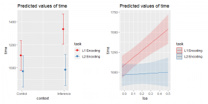
## plot
# Fixed-effectのみを描画する場合はtype = "eff"
# Interactionを描画する場合はtype = "int"
# Fixed-effectがカテゴリー変数の場合
p1 <-
plot_model(
model.a, type = "int", facet.grid = F,
title = "", fill.alpha = 0.8, geom.size = 1, show.ci = T
)
# Fixed-effectが連続変数の場合
p2 <-
plot_model(
model.b, type = "int", facet.grid = F,
title = "", fill.alpha = 0.8, geom.size = 1, show.ci = T
)
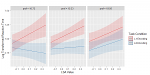
# Three-Way Interaction (Mean±1SD法)
p3 <-
plot_model(
model.c, type = "int", facet.grid = F,
title = "", legend.title = "Task Condition",
fill.alpha = 0.8, geom.size = 1, show.ci = T, mdrt.values = "meansd"
)
p3 + labs(x = "LSA Value", y = "Log Transformed Reaction Time")