Random Decision Forest

データセットの準備

library (randomForest)
# データの概要
   DV1 DV2 DV3 DV4 DV5 DV6 DV7 DV8 DV9 IV
1  0   0   4   4   4   5   5   5   5   4
2  0   0   4   5   5   5   5   5   5   5
3  0   0   4   4   4   5   3   4   4   5
4  0   0   4   5   4   3   5   5   5   5
5  0   0   5   4   2   5   5   5   5   5
6  0   0   4   4   4   4   4   4   4   4
# ランダムサンプリングの結果（乱数）を固定
set.seed (100)
# データのx%を抽出しトレーニング・テストデータに分ける
smpl <- sample(nrow(dat), 0.3*nrow(dat))
train <- dat[smpl, ]
test <- dat[-smpl, ]
# データセットを説明変数と予測変数に分ける
features <- train[1 : 9]
labels <- train[10]
# 予測変数をファクターに変換する（カテゴリ変数の場合）
labels <- as.factor(labels[[1]])

モデルを作成する

# Model Description
rf.model <- randomForest(x = features, y = labels, importance = TRUE, proximity = TRUE)

結果の可視化

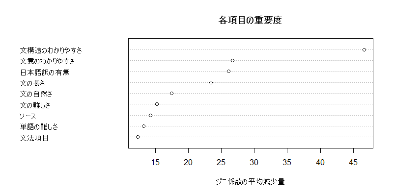
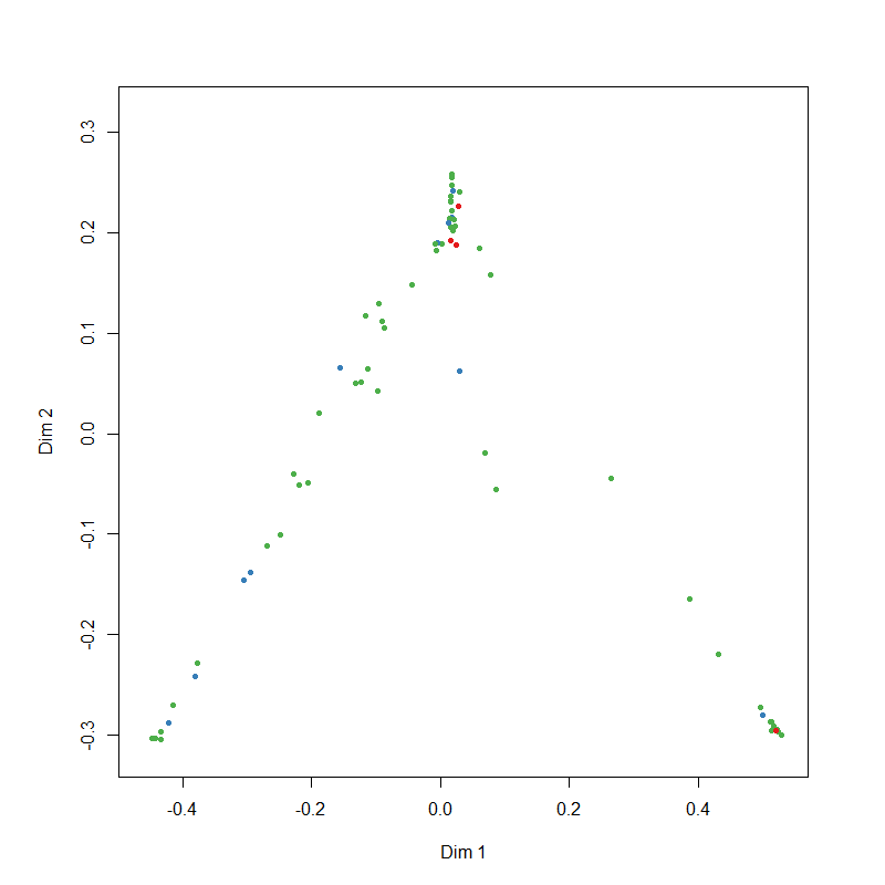
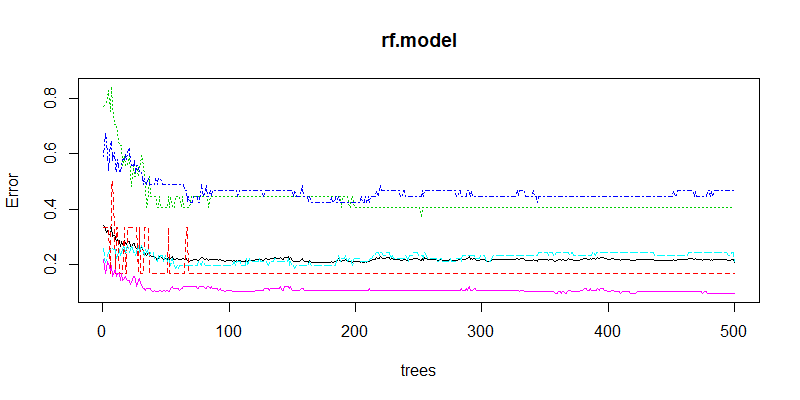
# 説明変数の重要度を表示・プロットする
imp <- importance(rf.model, scale = FALSE)
print(imp, digits = 4)
dotchart(sort(imp [, 7]), xlab = "ジニ係数の平均減少量", ylab = "", main = "各項目の重要度")
# 予測変数内の類似度を多次元尺度法で図示
MDSplot(rf.model, dat$IV)
# 機械学習の収束状況をプロット
plot(rf.model)

最適な特徴量とtreeの数を調べてモデルを再構築

rfTuning <- tuneRF(x = features, y = labels, stepFactor = 2, improve = 0.05, trace = TRUE, plot = TRUE, doBest = TRUE)
rf.model2 <- randomForest(
  x = features, 
  y = labels,  
  mtry = 6,        #エラーの最も低いmtry数を指定
  ntree = 200,     #モデルが収束したntreeを指定
  importance = T
  )
# 分類の正確さの確認
prdct <- predict(rf.model2, newdata = test)
table(prdct, test$IV)
correctAns <- 0
  for (i in 1:nrow (table (prdct, test$IV)))
correctAns <- correctAns + table (prdct, test$IV) [i, i]
correctAns/nrow (test)